Simple Method for Distance to Ellipse

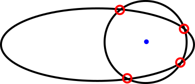
Analytically finding the smallest distance between a point and an ellipse boils down to solving a quartic equation. The easiest way to see this is by considering that a circle can intersect an ellipse at most four times. In this view, the problem is to find the circle that intersects the ellipse once. If formulated as a quartic, two of the roots will be shared at the intersection, and the other two roots will be complex.

Although a closed solution to the quartic does exist, it is unsurprising that iterative methods would be easier to implement and less prone to numeric instabilities. Generic root finders will work, but a robust implementation would be advised. This StackOverflow post shows what can go wrong when using a naive implementation of Newton's Method. Specialised iterative methods also exist, such as described by Maisonobe.

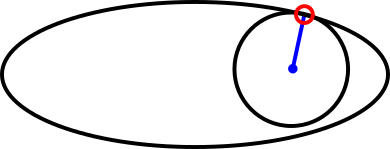
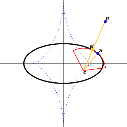
The paper's premise is that an oversized circle will intersect the ellipse at least two times. The iteration to minimise the distance between point a on the ellipse and p is as follows:

1. Choose a point a on the ellipse
2. Compute the distance r between a and p
3. On the circle centred at p with radius r, find the other intersection b
4. Set a' to the midpoint of a and b on the ellipse
5. Return to step 2

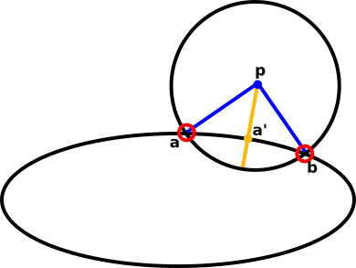
Visually a' is obviously a very good innovation over a, however computing b and a' is non trivial. In brief, the quartic still has 4 roots, but because the initial guess a is a solution, the quartic can be reduced to a cubic. The cubic is solved to find b. An additional quadratic is then solved to find a'. As noted, this complexity buys a very good estimate for a', and therefore the paper's claim that this algorithm is robust and converges quickly is very believable. What follows is an alternative, much simpler computation for a'.

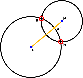
Consider the previous algorithm when the ellipse is a circle. a' then trivially lies on the line between c and p. It can also be seen that a' is optimal. The idea will become to locally approximate the ellipse as a circle, but first we must touch on curvature.

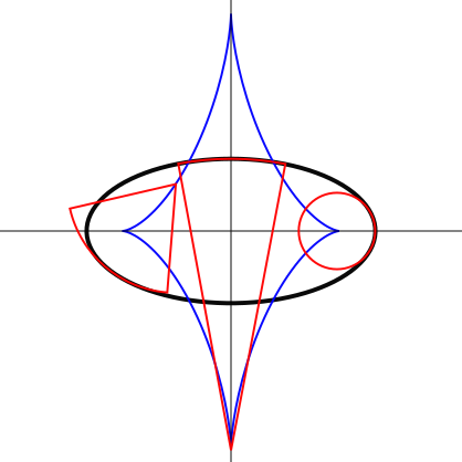
As a smooth curve, every point on the ellipse has a perpendicular normal. Additionally, every point has a radius of curvature. Without going into specifics, a tighter curve will result in a smaller radius of curvature, while a shallow curve will result in a larger radius of curvature. The centre of curvature of point e on the ellipse is the centre of the circle with radius equal to the radius of curvature and perpendicular to the ellipse at e. In other words, it is the centre of the circle that locally approximates the ellipse at e. The centre of curvatures can be plotted to form the evolute of the ellipse, which Wolfram and Wikipedia are better suited to explain.

It's now time to define the curves mathematically. Although everything can derived in Cartesian coordinates, a parametric definition avoids infinities about the vertices. For the ellipse use the standard definition.

  x = a * cos(t)
  y = b * sin(t)

The ellipse evolute also has a parametric form.

 ev_x = (a*a-b*b)/a * cos^3(t)
 ev_y = (b*b-a*a)/b * sin^3(t)

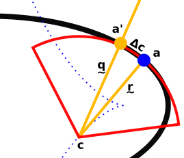
This is extremely useful for approximating the ellipse as a circle, since we know the centre of curvature for any t. Recall that when the ellipse is a circle, a' lies on the line between the circle centre c and p. Now modify this claim slightly, to state that a' lies on the line between the centre of curvature c and p. This is not as exact as the original a' from the paper since we've approximated the ellipse as a circle, but the beauty is that the closer we get to the optimal a', the better the approximation becomes. Therefore I would expect similar convergence and robustness properties.

Intersecting a line with an ellipse is a much simpler problem, however it still requires solving a quadratic. Since we're already estimating, an exact solution isn't required. From the previous figure, define two vectors r and q. Very loosely speaking, r is the radius of curvature and q intersects the ellipse where we would like the radius of curvature to have been. Since we are still using our circle approximation, we can compute the arc length between a and a' as the angle between r and q times the radius of curvature.

                (r x q)
  sin(Δc/|r|) ≈ -------
                |r||q|

Additionally, since Δc is small, we could further approximate by dropping the sine.

Now we would like to know how much to vary t by to achieve the same arc length delta on the ellipse. With a bit of calculus:

  dx/dt = -a * sin(t)
  dy/dt =  b * cos(t)
  dc/dt = sqrt((dx/dt)^2 + (dy/dt)^2)
  Δc/Δt ≈ sqrt(a^2 * sin^2(t) + b^2 * cos^2(t))
  Δt ≈ Δc / sqrt(a^2 * sin^2(t) + b^2 * cos^2(t))
  Δt ≈ Δc / sqrt(a^2 - a^2 * cos^2(t) + b^2 - b^2 * sin^2(t))
  Δt ≈ Δc / sqrt(a^2 + b^2 - x^2 - y^2)

  a'x = a * cos(t + Δt)
  a'y = b * sin(t + Δt)

This proves to be a good enough approximation, but it does suffer at the vertices (pointy ends) of the ellipse. Although in my experiments convergence was not affected, in the code listing I choose to confine t to the first quadrant and then correct the signs of the final result. For clarity, some obvious optimisations have been left unimplemented.

def solve(semi_major, semi_minor, p):
    px = abs(p[0])
    py = abs(p[1])

    t = math.pi / 4

    a = semi_major
    b = semi_minor

    for x in range(0, 3):
        x = a * math.cos(t)
        y = b * math.sin(t)

        ex = (a*a - b*b) * math.cos(t)**3 / a
        ey = (b*b - a*a) * math.sin(t)**3 / b

        rx = x - ex
        ry = y - ey

        qx = px - ex
        qy = py - ey

        r = math.hypot(ry, rx)
        q = math.hypot(qy, qx)

        delta_c = r * math.asin((rx*qy - ry*qx)/(r*q))
        delta_t = delta_c / math.sqrt(a*a + b*b - x*x - y*y)

        t += delta_t
        t = min(math.pi/2, max(0, t))

    return (math.copysign(x, p[0]), math.copysign(y, p[1]))

One remaining question is why t is initialised to a constant instead of atan2(py, px). This is only a good guess if p is outside of the ellipse. On the inside it is optimally bad. If p is inside the ellipse initialise to atan2(px, py). It turns out that a close to optimally bad guess will require additional iterations to move away from the initial guess in a random fashion. An optimally bad guess will get stuck. I've shown that for rather detailed reasons, the algorithm converges as long as you don't start near the optimally bad guess. You will be fine using atan2 if you correctly case for being inside or outside of the ellipse.

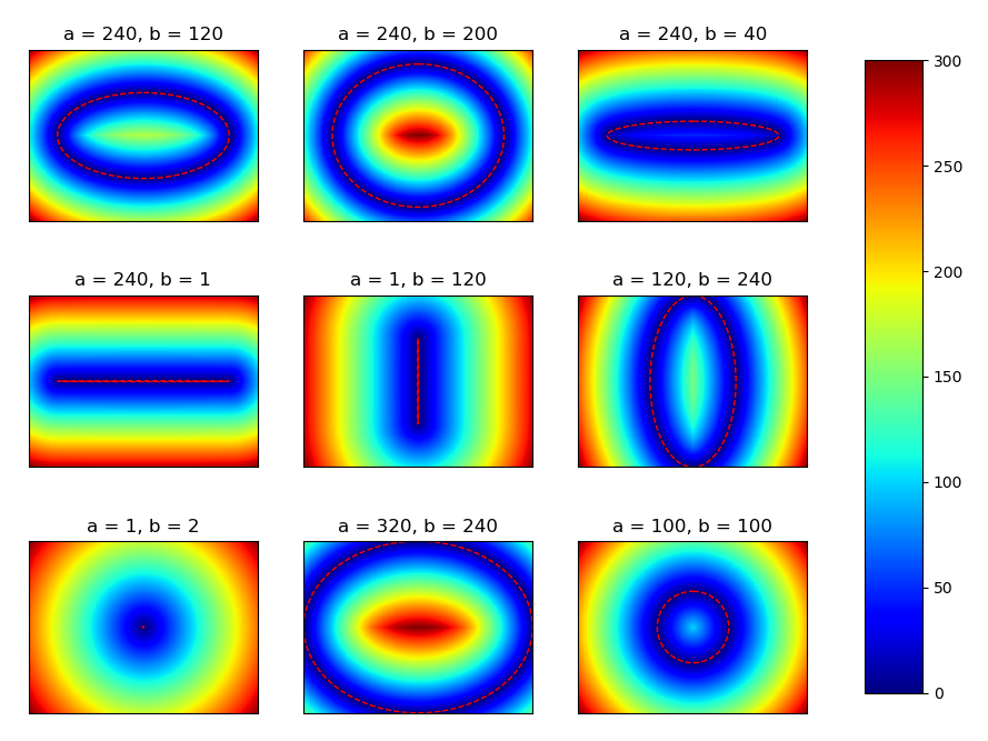
The plots show good convergence after three iterations over a wide range of eccentricities. However, at extreme eccentricities the algorithm will eventually fail. At some cutoff the ellipse should be considered a line.

The code for the plots is available on GitHub.